8.1 어텐션의 구조
- 어텐션 메커니즘을 사용하여 seq2seq에서 필요한 정보에만 '주목'할 수 있게 된다.
- 또한, seq2seq가 가지고 있던 문제도 해결할 수 있게 된다.
8.1.1 seq2seq의 문제점
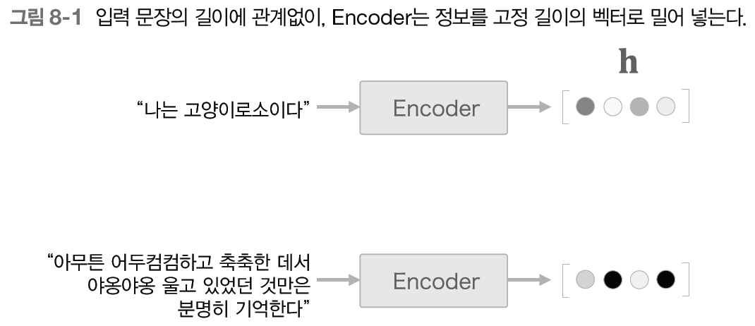
seq2seq에서는 Encoder가 시계열 데이터를 인코딩하고, 이 인코딩된 정보를 Decoder로 전달한다.
이때 Encoder의 출력은 '고정 길이 벡터'였는데, 이 부분에 큰 문제점이 있다.
고정 길이 벡터는 입력 데이터(문장)의 길이에 관계없이, 항상 같은 길이의 벡터로 변환한다.
그렇기 때문에, 필요한 정보가 벡터에 다 담기지 못한다.
8.1.2 Encoder 개선
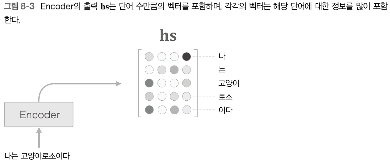
Encoder 출력의 길이를 입력 문장의 길이에 맞추어서 바꿔준다.
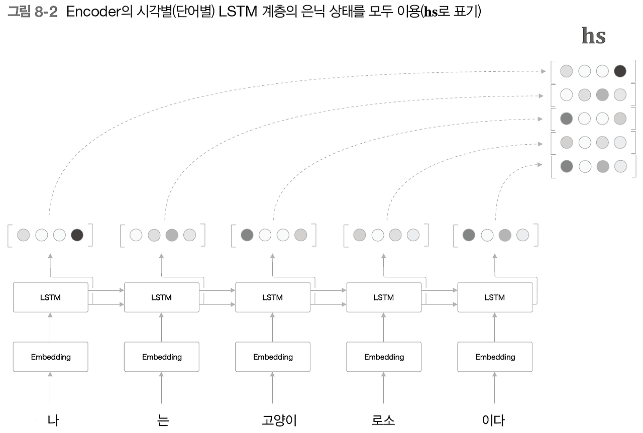
이제 마지막 은닉 상태뿐 아니라 각 시각(각 단어)의 은닉 상태 벡터를 모두 이용한다.
-> '하나의 고정 길이 벡터'라는 제약으로부터 해방됨
딥러닝 프레임워크에는 RNN 계열 계층을 초기화할때 '모든 시간의 은닉 상태 벡터 반환'과 '마지막 은닉 상태 벡터만 반환' 중 선택할 수 있게 하고 있다. 케라스는 return_sequences 이고, True면 모든 시각의 은닉 상태 벡터를 반환한다.
<파이토치>
파이토치의 RNN, LSTM, GRU 계층은 기본적으로 두 가지 출력을 반환한다.
- output: 모든 시간의 은닉 상태 벡터들을 포함한 텐서. 형태는 (seq_len, batch, num_directions * hidden_size)이며, 입력 시퀀스의 각 시간 단계에 대한 은닉 상태 벡터들이 포함됨
- h_n (hidden state): 마지막 은닉 상태 벡터. 형태는 (num_layers * num_directions, batch, hidden_size)
import torch
import torch.nn as nn

lstm = nn.LSTM(input_size=10, hidden_size=20, num_layers=2)
input_seq = torch.randn(5, 3, 10)  # (seq_len, batch, input_size)

output, (h_n, c_n) = lstm(input_seq)
<텐서플로우>
- 첫 번째 LSTM 계층의 출력: (batch_size, 10, 50) (모든 시간 단계에 대한 은닉 상태 벡터를 반환)
- 두 번째 LSTM 계층의 출력: (batch_size, 50) (두 번째 LSTM에서 마지막 시점의 은닉 상태 벡터만 반환)
from tensorflow.keras.models import Sequential
from tensorflow.keras.layers import LSTM, Dense

model = Sequential()
model.add(LSTM(50, input_shape=(10, 64), return_sequences=True))
model.add(LSTM(50, return_sequences=False))
model.add(Dense(1, activation='sigmoid'))

model.compile(optimizer='adam', loss='binary_crossentropy')
model.summary()
8.1.3 Decoder 개선 1
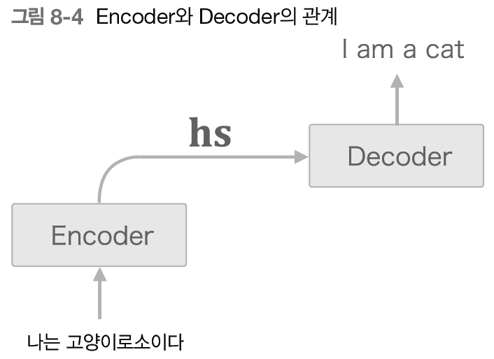
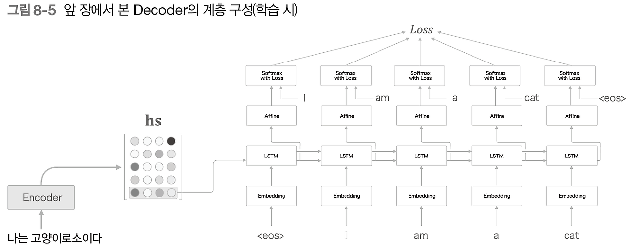
앞장에서는 hs의 마지막 줄만 빼네어서 디코더에 전달했음. -> hs전체를 다 활용할 수 있도록 디코더를 개선해보자.
우리가 번역을 할 때 나 = I, 고양이 = cat 이라는 얼라인먼트를 사용한다. 이러한 대응관계를 seq2seq에게 학습시킬 수 없을까?
우리의 목표: '도착어 단어'와 대응 관계에 있는 '출발어 단어'의 정보를 골라내는 것. 그리고 이 정보를 이용해 번역을 수행하는 것. 즉, 필요한 정보에만 주목하여 그 정보로부터 시계열 변환을 수행하는 것이 목표다. -> 그리고 이것이 어텐션
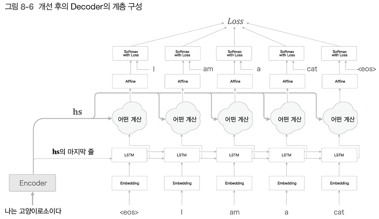
어떤 계산이 추가되었다.
어떤 계산의 입력: 1. 인코더로 부터 받는 hs 2. 시각별 LSTM계층의 은닉 상태.
어떤 계산의 출력: 필요한 정보만 골라 위쪽의 Affine계층으로 출력
결국 하고 싶은 것: 각 시각에서 디코더에 입력된 단어와 대응 관계인 단어 벡터를 hs에서 골라내기 <- 이걸 '어떤 계산'으로 하겠다는 것.
그런데 골라내기(선택)은 이산적 연산이므로 미분이 되지 않는다.
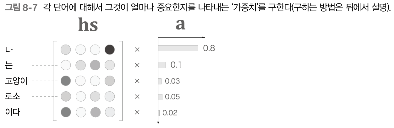
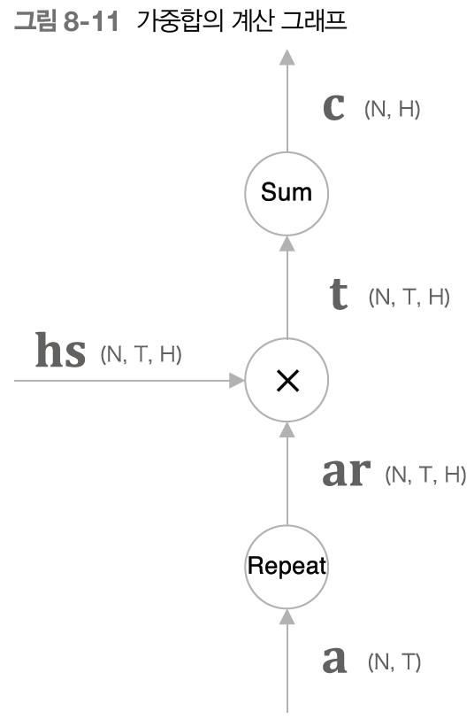
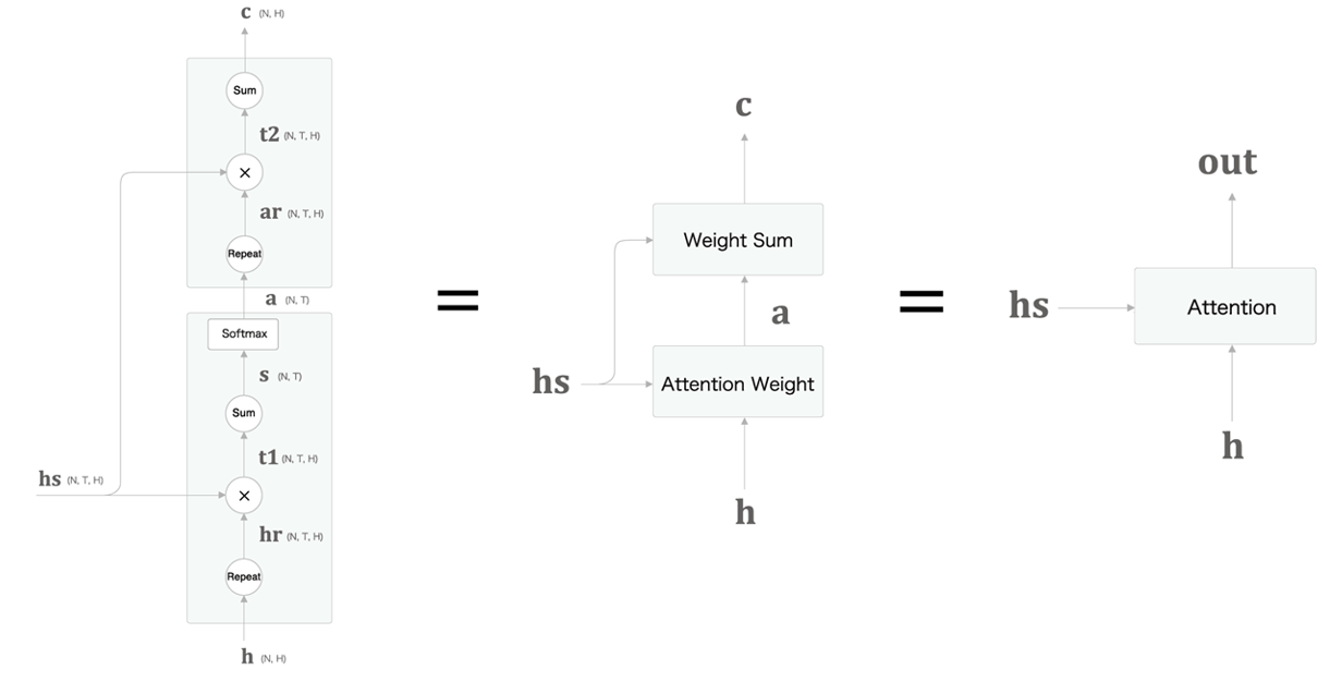
a는 각 단어의 중요도를 나타내는 가중치. 이 가중치와 hs를 가중합(weighted sum)을 하면 맥락 벡터가 구해진다.

대응하는 단어의 가중치가 가장 크면 맥락벡터에도 그 단어의 성분이 많이 포함되었다는 것. -> 선택하는 것을 대체한다.
가중합의 계산 그래프
- Repeat노드를 사용해 𝑎를 복제하고,
- 이어서 x 노드로 원소별 곱을 계산한 다음
- Sum노드로 합을 구한다.
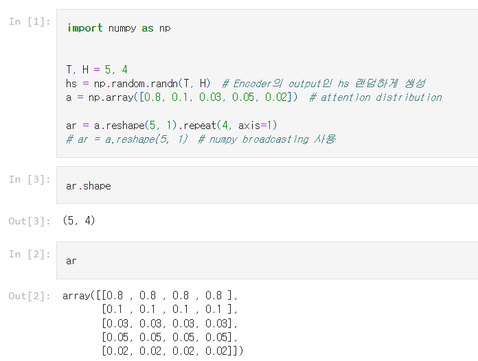
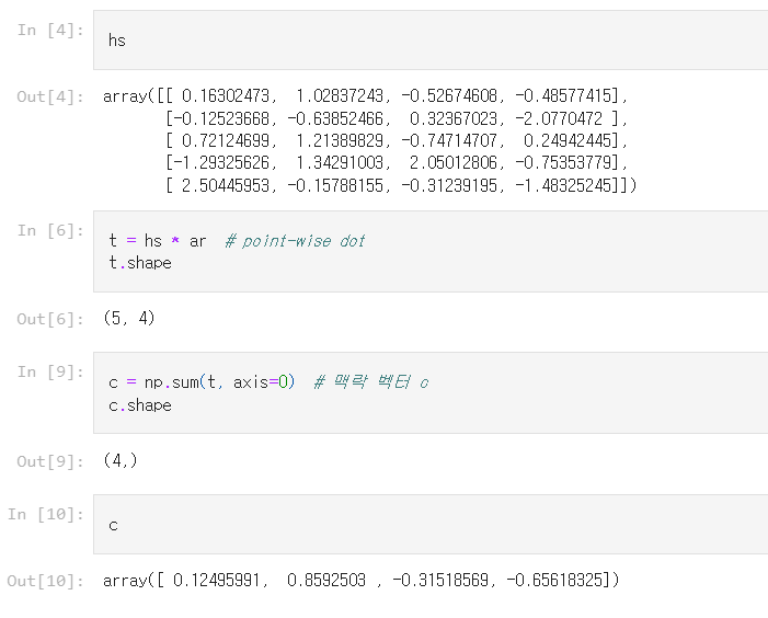
가중합 클래스 구현
import sys
sys.path.append('..')
from common.np import *
from common.layers import Softmax


class WeightSum:
    def __init__(self):
        self.params, self.grads = [], []
        self.cache = None

    def forward(self, hs, a):
        N, T, H = hs.shape

        ar= a.reshape(N, T, 1)#.repeat(H, axis=-1)
        t = hs * ar
        c = np.sum(t, axis=1)

        self.cache = (hs, ar)
        return c

    def backward(self, dc):
        hs, ar = self.cache
        N, T, H = hs.shape
        dt = dc.reshape(N, 1, H).repeat(T, axis=1)  # sum의 역전파 = repeat
        dar = dt * hs
        dhs = dt * ar
        da = np.sum(dar, axis=2)  # repeat노드에 대한 역전퍄 = sum

        return dhs, da
8.1.4 Decoder 개선 2
각 단어의 가중치 𝑎를 구하는 방법을 살펴보자. 데이터로부터 자동으로 학습하도록!
아래의 그림은 Decoder의 첫 번째 timestep에서의 LSTM 레이어가 hidden state를 출력하는 부분을 나타낸 것이다.
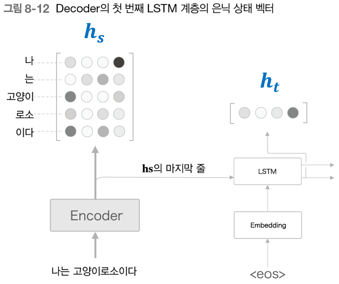
위의 그림에서 Encoder에서의 출력을 ℎ𝑠라 하고, Decoder의 LSTM의 출력(hidden state)을 ℎ𝑡라고 정의 했다.
Attention의 목표는 ℎ𝑡가 ℎ𝑠의 각 단어 벡터와 얼마나 '비슷한가'를 수치로 나타내는 것이다.
이를 나타내는 방법으로는 대표적으로 다음과 같이 3가지가 주로 사용된다.
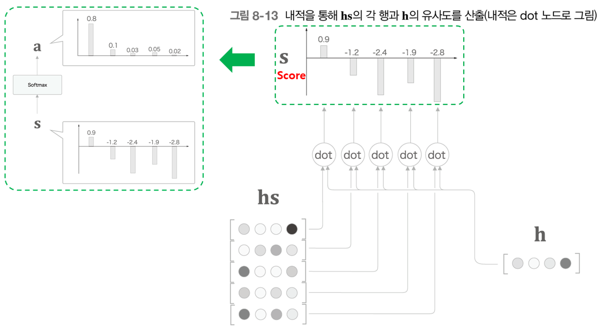
책에서는 가장 단순한 방법인 벡터의 '내적'을 이용한다.
두 벡터 𝑎=(𝑎1,𝑎2,⋯,𝑎𝑛)과 𝑏=(𝑏1,𝑏2,⋯,𝑏𝑛)의 내적은 다음과 같이 계산한다.
𝑎⋅𝑏=𝑎1𝑏1+𝑎2𝑏2+⋯+𝑎𝑛𝑏𝑛
'내적'의 직관적인 의미는 '두 벡터가 얼마나 같은 방향을 향하고 있는가'이다. 따라서, 두 벡터의 '유사도'를 표현하는 척도로 사용할 수 있다.
아래의 그림은 벡터의 내적을 이용해 유사도를 산출해내는 과정이다.
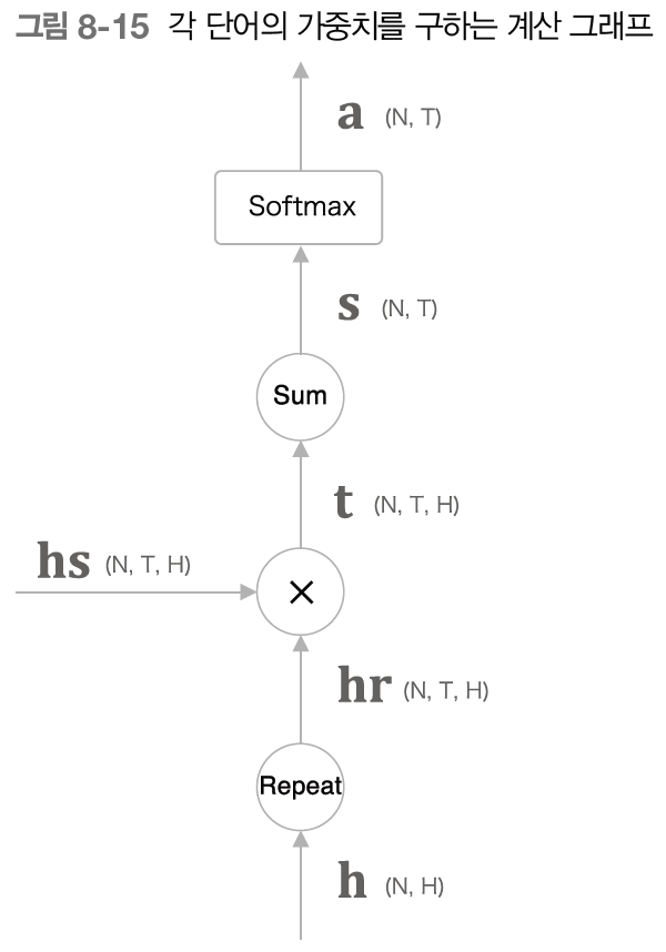
AttentionWeight 클래스
# chap08/attention_layer.py
import sys
sys.path.append('..')
from common.np import *  # import numpy as np
from common.layers import Softmax


class AttentionWeight:
    def __init__(self):
        self.params, self.grads = [], []
        self.softmax = Softmax()
        self.cache = None

    def forward(self, hs, h):
        N, T, H = hs.shape

        hr = h.reshape(N, 1, H)#.repeat(T, axis=1)
        t = hs * hr
        s = np.sum(t, axis=2)
        a = self.softmax.forward(s)

        self.cache = (hs, hr)
        return a

    def backward(self, da):
        hs, hr = self.cache
        N, T, H = hs.shape

        ds = self.softmax.backward(da)
        dt = ds.reshape(N, T, 1).repeat(H, axis=2)
        dhs = dt * hr
        dhr = dt * hs
        dh = np.sum(dhr, axis=1)

        return dhs, dh
8.1.5 Decoder 개선 3
8.1.4 에서 AttentionWeight계층, 8.1.3에서 Weight Sum 계층을 각각 구현했다. 이제 하나로 결합하자.
# chap08/attention_layer.py
import sys
sys.path.append('..')
from common.np import * # import numpy as np
from common.layers import Softmax
class Attention:
def __init__(self):
self.params, self.grads = [], []
self.attention_weight_layer = AttentionWeight()
self.weight_sum_layer = WeightSum()
self.attention_weight = None
def forward(self, hs, h):
a = self.attention_weight_layer.forward(hs, h)
out = self.weight_sum_layer.forward(hs, a)
self.attention_weight = a
return out
def backward(self, dout):
dhs0, da = self.weight_sum_layer.backward(dout)
dhs1, dh = self.attention_weight_layer.backward(da)
dhs = dhs0 + dhs1
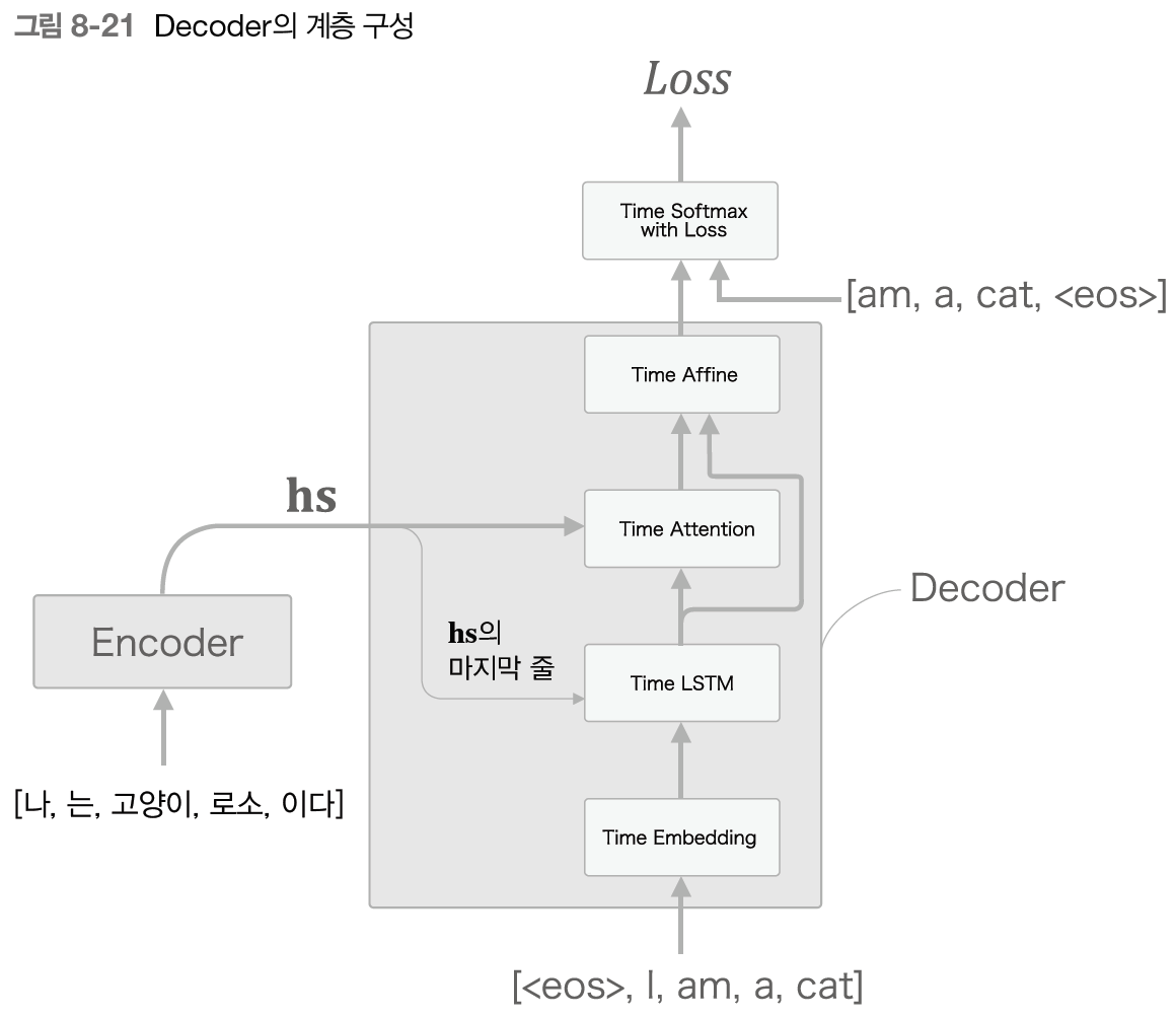
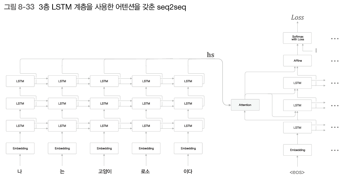
return dhs, dh어텐션 레이어가 반영된 seq2seq
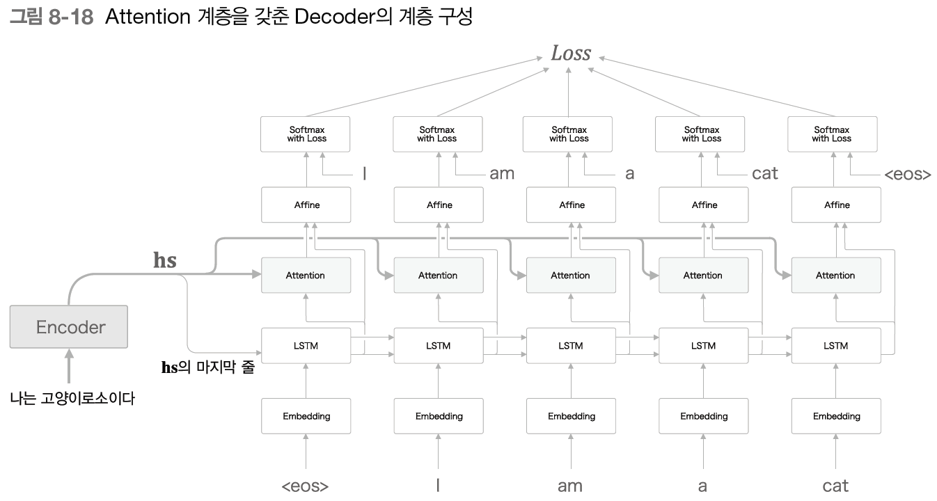
위의 그림에서 각 timestep 𝑡의 Attention레이어에는 Encoder의 출력인 hs가 입력된다.
그리고 Decoder에서 LSTM레이어의 hidden state ℎ𝑡 벡터를 Affine 레이어에 context 벡터와 concat하여 입력한다.
TimeAttention 구현
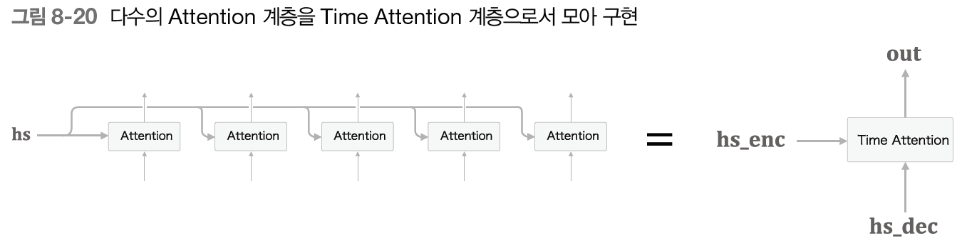
class TimeAttention:
    def __init__(self):
        self.params, self.grads = [], []
        self.layers = None
        self.attention_weights = None

    def forward(self, hs_enc, hs_dec):
        N, T, H = hs_dec.shape
        out = np.empty_like(hs_dec)
        self.layers = []
        self.attention_weights = []

        for t in range(T):
            layer = Attention()
            out[:, t, :] = layer.forward(hs_enc, hs_dec[:,t,:])
            self.layers.append(layer)
            self.attention_weights.append(layer.attention_weight)

        return out

    def backward(self, dout):
        N, T, H = dout.shape
        dhs_enc = 0
        dhs_dec = np.empty_like(dout)

        for t in range(T):
            layer = self.layers[t]
            dhs, dh = layer.backward(dout[:, t, :])
            dhs_enc += dhs
            dhs_dec[:,t,:] = dh

        return dhs_enc, dhs_dec
8.2 어텐션을 갖춘 seq2seq 구현
8.2.1 Encoder 구현
# chap08/attention_seq2seq.py
import sys
sys.path.append('..')
from common.time_layers import *
from seq2seq import Encoder, Seq2seq
from attention_layer import TimeAttention


class AttentionEncoder(Encoder):
    def forward(self, xs):
        xs = self.embed.forward(xs)
        hs = self.lstm.forward(xs)
        return hs

    def backward(self, dhs):
        dout = self.lstm.backward(dhs)
        dout = self.embed.backward(dout)
        return dout
8.2.2 Decoder 구현
class AttentionDecoder:
    def __init__(self, vocab_size, wordvec_size, hidden_size):
        V, D, H = vocab_size, wordvec_size, hidden_size
        rn = np.random.randn

        embed_W = (rn(V, D) / 100).astype('f')
        lstm_Wx = (rn(D, 4 * H) / np.sqrt(D)).astype('f')
        lstm_Wh = (rn(H, 4 * H) / np.sqrt(H)).astype('f')
        lstm_b = np.zeros(4 * H).astype('f')
        affine_W = (rn(2*H, V) / np.sqrt(2*H)).astype('f')
        affine_b = np.zeros(V).astype('f')

        self.embed = TimeEmbedding(embed_W)
        self.lstm = TimeLSTM(lstm_Wx, lstm_Wh, lstm_b, stateful=True)
        self.attention = TimeAttention()  # Attention 레이어
        self.affine = TimeAffine(affine_W, affine_b)
        layers = [self.embed, self.lstm, self.attention, self.affine]

        self.params, self.grads = [], []
        for layer in layers:
            self.params += layer.params
            self.grads += layer.grads

    def forward(self, xs, enc_hs):
        h = enc_hs[:,-1]
        self.lstm.set_state(h)

        out = self.embed.forward(xs)
        dec_hs = self.lstm.forward(out)
        c = self.attention.forward(enc_hs, dec_hs)  # context vector
        out = np.concatenate((c, dec_hs), axis=2)  # context_vector & lstm h_t
        score = self.affine.forward(out)

        return score

    def backward(self, dscore):
        dout = self.affine.backward(dscore)
        N, T, H2 = dout.shape
        H = H2 // 2

        dc, ddec_hs0 = dout[:,:,:H], dout[:,:,H:]
        denc_hs, ddec_hs1 = self.attention.backward(dc)
        ddec_hs = ddec_hs0 + ddec_hs1
        dout = self.lstm.backward(ddec_hs)
        dh = self.lstm.dh
        denc_hs[:, -1] += dh
        self.embed.backward(dout)

        return denc_hs

    def generate(self, enc_hs, start_id, sample_size):
        sampled = []
        sample_id = start_id
        h = enc_hs[:, -1]
        self.lstm.set_state(h)

        for _ in range(sample_size):
            x = np.array([sample_id]).reshape((1, 1))

            out = self.embed.forward(x)
            dec_hs = self.lstm.forward(out)
            c = self.attention.forward(enc_hs, dec_hs)
            out = np.concatenate((c, dec_hs), axis=2)
            score = self.affine.forward(out)

            sample_id = np.argmax(score.flatten())
            sampled.append(sample_id)

        return sampled
8.2.3 seq2seq 구현
class AttentionSeq2seq(Seq2seq):
    def __init__(self, vocab_size, wordvec_size, hidden_size):
        args = vocab_size, wordvec_size, hidden_size
        self.encoder = AttentionEncoder(*args)
        self.decoder = AttentionDecoder(*args)
        self.softmax = TimeSoftmaxWithLoss()

        self.params = self.encoder.params + self.decoder.params
        self.grads = self.encoder.grads + self.decoder.grads
8.3 어텐션 평가
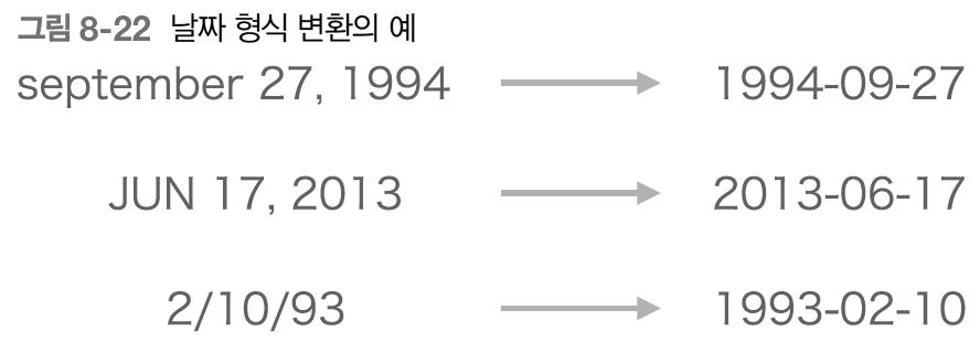
8.3.1 날짜 형식 변환 문제
8.3.2 어텐션을 갖춘 seq2seq의 학습
import sys
sys.path.append('..')
import numpy as np
import matplotlib.pyplot as plt
import matplotlib
import matplotlib.font_manager as fm
font_path = 'C:/Windows/Fonts/malgun.ttf'
font_name = fm.FontProperties(fname=font_path, size=10).get_name()
plt.rc('font', family=font_name, size=12)
from dataset import sequence
from common.optimizer import Adam
from common.trainer import Trainer
from common.util import eval_seq2seq
from attention_seq2seq import AttentionSeq2seq
from seq2seq import Seq2seq
from peeky_seq2seq import PeekySeq2seq


# 데이터 읽기
(x_train, t_train), (x_test, t_test) = sequence.load_data('date.txt')
char_to_id, id_to_char = sequence.get_vocab()

# 입력 문장 반전
x_train, x_test = x_train[:, ::-1], x_test[:, ::-1]

# 하이퍼파라미터 설정
vocab_size = len(char_to_id)
wordvec_size = 16
hidden_size = 256
batch_size = 128
max_epoch = 10
max_grad = 5.0

model = AttentionSeq2seq(vocab_size, wordvec_size, hidden_size)
# model = Seq2seq(vocab_size, wordvec_size, hidden_size)
# model = PeekySeq2seq(vocab_size, wordvec_size, hidden_size)

optimizer = Adam()
trainer = Trainer(model, optimizer)

acc_list = []
for epoch in range(max_epoch):
    trainer.fit(x_train, t_train, max_epoch=1,
                batch_size=batch_size, max_grad=max_grad, eval_interval=150)

    correct_num = 0
    for i in range(len(x_test)):
        question, correct = x_test[[i]], t_test[[i]]
        verbose = i < 10
        correct_num += eval_seq2seq(model, question, correct,
                                    id_to_char, verbose, is_reverse=True)

    acc = float(correct_num) / len(x_test)
    acc_list.append(acc)
    print('정확도 %.3f%%' % (acc * 100))


model.save_params()

# 그래프 그리기
x = np.arange(len(acc_list))
plt.plot(x, acc_list, marker='o')
plt.xlabel('에폭')
plt.ylabel('정확도')
plt.ylim(-0.05, 1.05)
plt.show()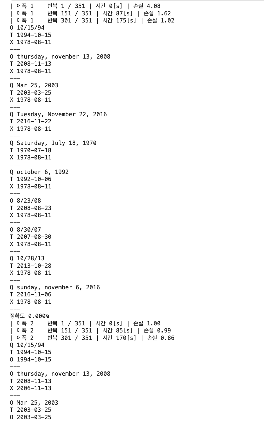
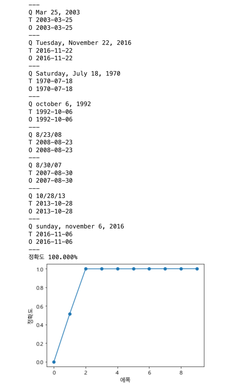
다른 모델 (앞 장의 seq2seq, seq2seq+peeky)과 비교해보면 빠르게 정확도가 올라간다.
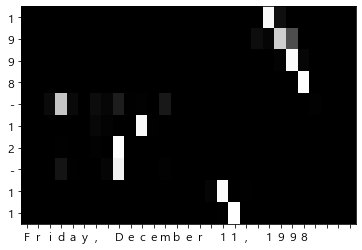
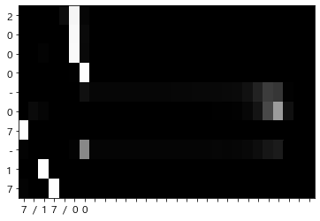
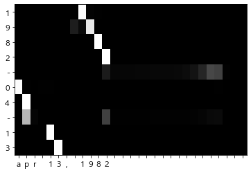
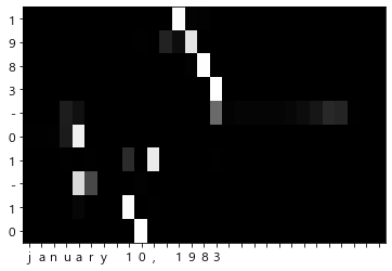
8.3.3 어텐션 시각화
import sys
sys.path.append('..')
import numpy as np
from dataset import sequence
import matplotlib.pyplot as plt
import matplotlib
import matplotlib.font_manager as fm
font_path = 'C:/Windows/Fonts/malgun.ttf'
font_name = fm.FontProperties(fname=font_path, size=10).get_name()
plt.rc('font', family=font_name, size=12)

from attention_seq2seq import AttentionSeq2seq


(x_train, t_train), (x_test, t_test) = \
    sequence.load_data('date.txt')
char_to_id, id_to_char = sequence.get_vocab()

# 입력 문장 반전
x_train, x_test = x_train[:, ::-1], x_test[:, ::-1]

vocab_size = len(char_to_id)
wordvec_size = 16
hidden_size = 256

model = AttentionSeq2seq(vocab_size, wordvec_size, hidden_size)
model.load_params()

_idx = 0
def visualize(attention_map, row_labels, column_labels):
    fig, ax = plt.subplots()
    ax.pcolor(attention_map, cmap=plt.cm.Greys_r, vmin=0.0, vmax=1.0)

    ax.patch.set_facecolor('black')
    ax.set_yticks(np.arange(attention_map.shape[0])+0.5, minor=False)
    ax.set_xticks(np.arange(attention_map.shape[1])+0.5, minor=False)
    ax.invert_yaxis()
    ax.set_xticklabels(row_labels, minor=False)
    ax.set_yticklabels(column_labels, minor=False)

    global _idx
    _idx += 1
    plt.show()


np.random.seed(1984)
for _ in range(5):
    idx = [np.random.randint(0, len(x_test))]
    x = x_test[idx]
    t = t_test[idx]

    model.forward(x, t)
    d = model.decoder.attention.attention_weights
    d = np.array(d)
    attention_map = d.reshape(d.shape[0], d.shape[2])

    # 출력하기 위해 반전
    attention_map = attention_map[:,::-1]
    x = x[:,::-1]

    row_labels = [id_to_char[i] for i in x[0]]
    column_labels = [id_to_char[i] for i in t[0]]
    column_labels = column_labels[1:]

    visualize(attention_map, row_labels, column_labels)
8.4 어텐션에 관한 남은 이야기
8.4.1 양방향 RNN
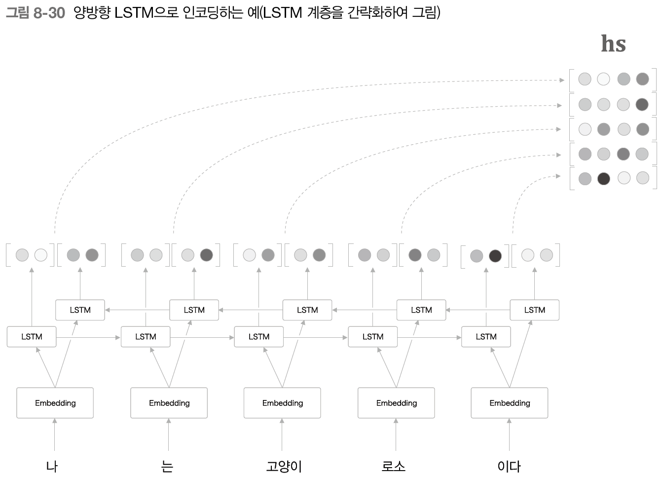
Bidirectional RNN(LSTM, GRU 등)에서는 정방향 LSTM 레이어에 역방향 으로 처리하는 LSTM 레이어를 추가한 형태를 말한다.
그리고, 각 timestep 𝑡에서 정방향 & 역방향 LSTM의 hidden state ℎ𝑡를 연결(concat, 또는 sum, average 등)시킨 벡터를 최종 ℎ𝑡로 만든다.
양방향으로 처리함으로써, 각 단어에 대응하는 hidden state 벡터에는 forward, backward 방양으로부터의 정보를 집약할 수 있다.
TimeBiLSTM
# common/time_layers.py

class TimeBiLSTM:
    def __init__(self, Wx1, Wh1, b1,
                 Wx2, Wh2, b2, stateful=False):
        self.forward_lstm = TimeLSTM(Wx1, Wh1, b1, stateful)
        self.backward_lstm = TimeLSTM(Wx2, Wh2, b2, stateful)
        self.params = self.forward_lstm.params + self.backward_lstm.params
        self.grads = self.forward_lstm.grads + self.backward_lstm.grads

    def forward(self, xs):
        o1 = self.forward_lstm.forward(xs)
        o2 = self.backward_lstm.forward(xs[:, ::-1])  # backward를 위해 입력데이터 반전
        o2 = o2[:, ::-1]

        out = np.concatenate((o1, o2), axis=2)  # forward, backward concat
        return out

    def backward(self, dhs):
        H = dhs.shape[2] // 2
        do1 = dhs[:, :, :H]
        do2 = dhs[:, :, H:]

        dxs1 = self.forward_lstm.backward(do1)
        do2 = do2[:, ::-1]
        dxs2 = self.backward_lstm.backward(do2)
        dxs2 = dxs2[:, ::-1]
        dxs = dxs1 + dxs2
        return dxs
8.4.2 Attention 계층 사용 방법
Attention 레이어는 다양하게 조합되어 사용할 수 있다.
다만, Attention 레이어를 조합하였을 때, 정확도에 대한 영향은 직접 데이터를 사용해 검증해보지 않으면 모른다.
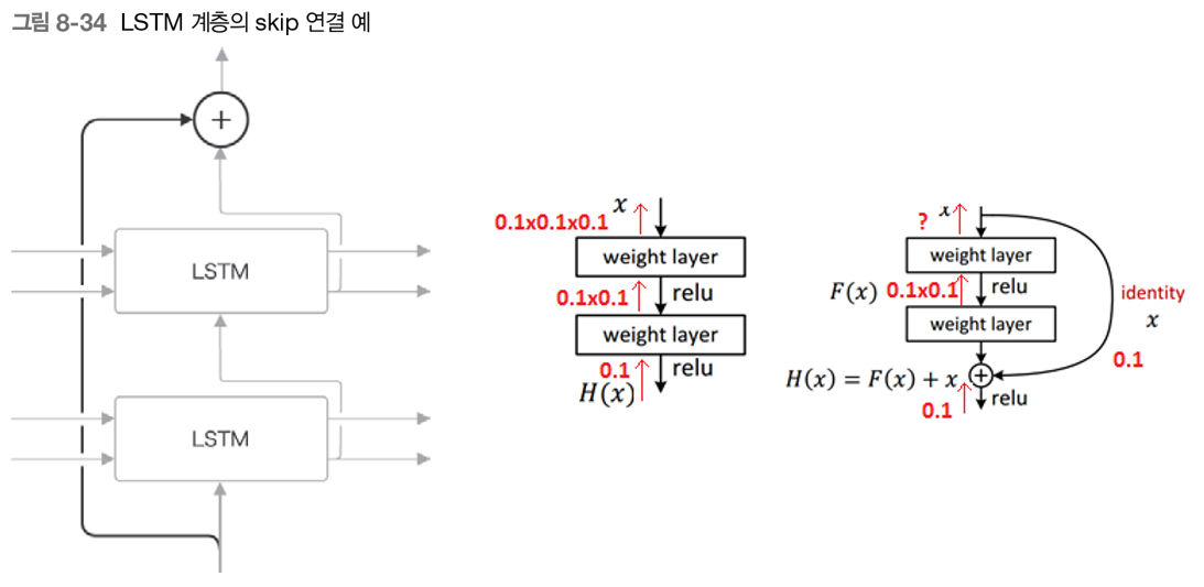
8.4.3 seq2seq 심층화와 skip 연결
번역 등 현실에서의 애플리케이션들은 풀어야 할 문제가 훨씬 복잡하다.
이럴 경우에 층을 깊게 쌓은 seq2seq를 사용할 수 있다.
층을 깊게 쌓을 때 사용되는 중요한 기법 중에 skip connection이 있다(residual connection 또는 short-cut).
skip connection에서는 2개의 출력이 하나로 '더해'지기 때문에 역전파 시 기울기가 '그대로 흘려' 보낸다.
따라서, 층이 깊어져도 기울기 소실(또는 폭발)이 되지 않고 전파되어, 좋은 학습을 기대할 수 있다.
8.5 어텐션 응용
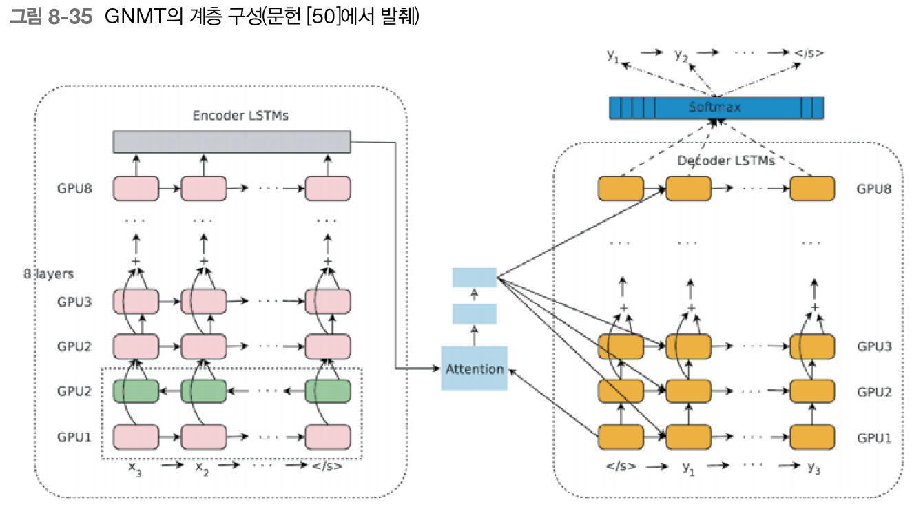
8.5.1 구글 신경망 기계 번역(GNMT)
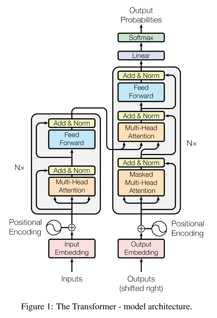
8.5.2 트랜스포머
8.6 정리
- 번역이나 음성 인식 등, 한 시계열 데이터를 다른 시계열 데이터로 변환하는 작업에서는 시계열 데이터 사이의 대응 관계가 존재하는 경우가 많다.
- 어텐션은 두 시계열 데이터 사이의 대응 관계를 데이터로부터 학습한다.
- 어텐션에서는 (하나의 방법으로서) 벡터의 내적을 사용해 벡터 사이의 유사도를 구하고, 그 유사도를 이용한 가중합 벡터가 어텐션의 출력이 된다.
- 어텐션에서 사용하는 연산은 미분 가능하기 때문에 오차역전파법으로 학습할 수 있다.
- 어텐션이 산출하는 가중치(확률)을 시각화하면 입출력의 대응 관계를 볼 수 있다.
'ML & DL > 책 & 강의' 카테고리의 다른 글
| [나는 리뷰어다] AI를 위한 필수 수학 (3) | 2024.09.29 |
|---|---|
| [나는 리뷰어다] AI 딥 다이브 (0) | 2024.08.25 |
| [C언어로 쉽게 풀어 쓴 자료구조] 1 자료구조와 알고리즘 (0) | 2024.08.11 |
| [밑시딥2] CHAPTER 6 게이트가 추가된 RNN (0) | 2024.07.29 |
| [나는 리뷰어다] 실무로 통하는 타입스크립트 (1) | 2024.07.28 |


댓글